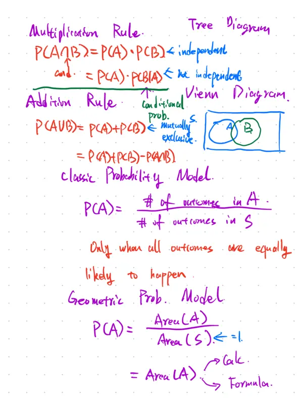
Multiplication Rule. Tree Diagram P(A∩B)=P(A) • P(B) independent cond. = P(A) • P(B|A) not independent → Venn Diagram. Addition Rule Conditional prob. P(A∪B) = P(A)+P(B) mutually exclusive. A B = P(A)+P(B)-P(A∩B) Classic Probability Model. P(A)= # of outcomes in A. / # of outcomes in S Only when all outcomes are equally likely to happen Geometric Prob.. Model. P(A)= Area(A) / Area(S)=1. = Area(A) → Calc. Formula. Calculation of conditional prob. P(B|A) = P(A∩B) / P(A). → Bayes Formula. Definition of independent. P(B|A)=P(B). P(A∩B)=P(A) • P(B). Mutually. Exclusive. 互斥. A∩B=Φ. P(A∩B)=0. no overlap. 独立一定不互斥。 互斥一定不独立 Probability Rule 1) Range of Prob. 0 ≤ P ≤ 1 2). Prob. of all outcomes is 1. 3). Complement Rule. P(Aᶜ) = 1-P(A) Prob for a single event. 1) equally likely outcomes Classic Prob. Model. P(A) = # of outcomes in A / # of outcomes in S or # of total outcomes Think about fair coin toss, roll dice.... 2) Outcomes are not equally likely or infinite number of outcomes. Geometric Prob. model.. P(A) = Area(A) / Area(S) Prob. for 2 event Weighted coin = Area(A). 0.7 H 0.7 H HH 0.49 0.3 T HT 0.21 H TH. 0.21 0.3 T TT. 0.09 HH 0.49 B={TH, TT} HT 0.21 TH 0.21 TT 0.09 = 0.21+0.09 Aᶜ A∩B A∪B A|B. multiplication rule P(A∩B) = P(A) • P(B|A) = P(B) • P(A|B). General addition rule P(A∪B) = P(A)+P(B)-P(A∩B). General P(A|B) = P(A∩B) / P(B). Bayes formula 条件是分母,相交是分子 Independent When Independent P(A|B)=P(A). <=> P(A∩B) = P(A) • P(B) Mutually exclusive. when M.E. P(A∩B)=0 <=> P(A∪B) = P(A)+P(B) Random Event => Random Variable. Random Variable Categorical Quantitative. {X=1.5, 1.5 ≤ X ≤ 1.8} {X=Red} Event A B. C P(C) → cal like before with Prob. model P(A) & P(B) {X→ generic distribution {X→ special distribution X→ generic distribution P(1.5 ≤ X < 1.6) 1.5-1.6 108 = 108 / 337 1.6-1.7 121. 1.8-1.9 88 1.9- 20 209 128 337 P(X=1.5). X→ Special Distributions → discrete → binomial → geometric continuous → normal → uniform. Random Variable X. parameters E(X). Expected Value. aka. Mean. 期望值 均值 defn: E(X) = Σ xi pi μx X | 0 | 1 | 2 | 3 Pi | 0.3 | 0.2 | 0.1 | 0.4 μx = E(X) = 0x0.3 + 1x0.2 + 2x0.1 + 3x0.4 = 1.6 It's the center of distribution of. X. How to interprete. 1.6. expected value for X. Statement: The expected height for random selected girls of HW is 1.62m How to interpret the 1.62m expected Value. After repeated trials of randomly selecting girls and take their height the long run average of girls height is. 1.62m. Standard Deviations / Variances of Random variable σx² = Var(X) = Σ (xi - E(X))² Pi = Σ (xi - E(X))² / n (不记) σx = Std(X) = √[Σ (xi - E(X))² Pi] Define X is the height of randomly selected girl in HW. The std of x is 5 cm. interpret the meaning of std. After many many trials of randomly selecting girls in HW and measure her height, the typical distance between their height and the mean of their height is 5 cm