Class: AP1 | Unit: Unit 4 | Updated: 2026-02-09
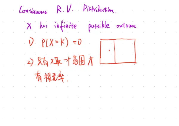
Continuous R.V. Distribution. X has infinite possible outcome. P(X=K) = 0. Only by taking a range can there be a probability. Special distributions for Continuous R.V. 1) uniform distribution. area=1. P(k1 <= X <= k2) = (k2 - k1) / (b-a). E(X)=(b-a)/2. Std(X) = (b-a)/sqrt(12). Note: area = proportion = probability = percentage/percentile. 2) normal distribution. Given other values, find area. Use normalcdf. Given area, find other values. Use invNorm. Z=ax+by+c. Z=aX. E(Z) = E(ax+by+c) = E(aX)+E(bY)+E(C) = aE(X)+bE(Y)+C. Var(Z) = Var(ax+by+c) = Var(aX) + Var(bY) + Var(C) = a^2 Var(X) + b^2 Var(Y) (Var(C)=0). Std(Z) = sqrt(Var(Z)) = sqrt(a^2 Var(X) + b^2 Var(Y)) = sqrt(a^2 Std^2(X) + b^2 Std^2(Y)). Var(X) = sum[pi * (xi - mu_X)^2] (where xi - mu_X is deviation). Std(X) = sqrt(Var(X)). Y = 0.54M + 0.46W. E(Y) = 0.54 * E(M) + 0.46 * E(W). Example: 54% M has mean 20.7, 46% W has mean 20.2. So E(Y) = 0.54 * 20.7 + 0.46 * 20.2. Calculation example: 150+50 * [0.05*1 + 0.1*2 + 0.22*3 + 0.3*4 + 0.18*5 + 0.12*6 + 0.03*7] = 150+50*3.97 = 347. For a linear transformation Z=aX: E(Z) = E(aX) = aE(X). Std(Z) = sqrt(a^2 * Std^2(X)) = |a| * Std(X). Example: W = 7+2X. E(W) = E(7+2X) = 7+2E(X). If E(X)=12, then E(W) = 7+2*12 = 31. Std(W) = Std(7+2X) = Std(2X) = |2| * Std(X). If Std(X)=3, then Std(W) = 2*3 = 6. Given E(D)=2.6 and Var(D)=3.6. For P related to D, Std(P) = Std(1.5D). For the difference of two independent random variables C=A-B: We want to find P(A-B > 0). The expected value E(C) = E(A-B) = E(A) - E(B). Example result: E(C) = -15. The standard deviation Std(C) = sqrt(Std^2(A) + Std^2(B)) = 33.54 (assuming A and B are independent). To find P(C>0) using a normal distribution, use normalcdf(lower_bound=0, upper_bound=1e99, mean=-15, standard_deviation=33.54).
